
Instagram passes through a ConvNet
After moving to India last year, I decided to be more active on Instagram, post lots of pictures of my endeavors in my home country. This has been a great way to document my life in New Delhi and travels around the country.
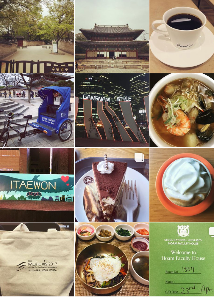
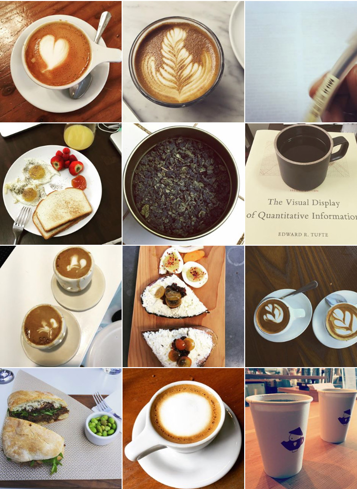
Over time, I have posted more than 500 pictures on Instagram that also include my earlier posts from my life in the US, travels in Europe, and short trips visiting my parents in India. I would like to believe that my instagram is a good indicator of my lifestyle, my interests, and aspirations.
In fact my instagram bio reads -
In this exercise, I try to analyze all the images that I've posted on the instagram till November 2017, this excludes videos and stories.
The goal of this exploration is to find motifs in my pictures, though a quick glance through my posts can yeild prominent themes in these pictures. A friend once claimed to guess the topic of my next post in less than 3 attempts(!).
Instead of a human, the plan is to have the machine go through these images to find hidden chacteristics in them, and group them based on the learned motifs. We have the tools from machine learning at our disposal, especially the current paradigm of deep neural networks which has shown great success in image analysis. In fact, this post is motivated by my interest in deep convolution neural networks.
Thus the refined goal is to automatically confirm the known motifs and identify some unknown ones.
The data consists of 526 images extracted from instagram using the Instaport app.
We cast the images into vectors, called features in machine learning lingo. Any image can be defined by the values of the Red, Green, and Blue (RGB) color channels contributing to each pixel. Each image in this data has (640 * 640) pixels, and thus the vector of RGB channels, called raw features, is of the dimension (640 * 640) * 3. These are very high-dimensional vectors, we will reshape these into (150*150)*3 dimensional features for further analysis.
Features that we have extracted for our images are very high-dimensional, and it's not possible to visualize them directly. Fortunately, there are methods to project higher-dimensional spaces onto lower dimensions such that the new space retains the intricaces of the relationships among the data points as much as possible.
One of the most popular dimensional-reduction techniques is t-distributed Stochaistic Neighbor Embedding(tsne), which is particularly effective for visualizing high-dimensional data by embedding the data into a 2-dimensional space. This technique casts relationships between data points to joint probability distributions, and then tried to find the low-dimensional representation such that a suitable measure of distance (e.g. Kullback-Leibler divergence) between the higher-dimensional and the lower-dimensional joint probabilities.
We will employ an implementation from the python scikit-learn package.
It is important to note that the reduced features loose any meaning, and they do not lend themselves to any obvious interpretation. The primary goal is to preserve the proximity relation between the points to be able to visualize them.
To further explore the data and find possible groups among images, the raw features are clustered using the K-Means algorithm. This is the most popular clustering algorithm which starts with k random data points as intial centroids of the clusters, assign points to the nearest centroid, choose new centroid as the mean of the points in the clusters and repeat until a stopping criterion (Lloyd's optimization).
It is a very general purpose algorithm, which has shown success in many cases, although a big hindrance to its practical adaptability is the requirement of the apriori knowledge of the number of clusters (k parameter).
In this current study, based on the exploration of the data, and the authors knowledge of his instagramming activity, k is chosen to be 10. I would like to admit that better choice of a clustering algorithm, and the parameters is surely possible via deep dive into the data and statistical analysis.
The raw features from the color channels were not very effective in capturing the intricacies of the images. Following the philosophy of machine learning, we would want to transform the data into a new space with the hope that the transformed data will be more suited to the task at hand, this is known as feature engineering in machine learning literature.
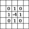
We will learn refined features by passing the images through an artificial neural network (ANN), which is a machine learning technique loosely modeled on the functioning of human brain. Essentially, an ANN is a set of units, appropriately called a neurons, which are organized in different layers. There are connections between neurons for transmitting signal, which usually flows from one layer to next. Each neuron gathers information from the neurons feeding into it, process it (a non-linear function followed by linear combination of the input signals), and passes on to a neuron in the next layer.
Source: Denny Britz, WildML (Post)
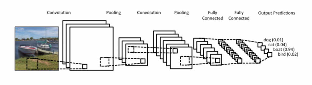
Source: Denny Britz, WildML (Post)
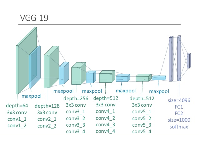
These high-level features extracted from the VGG19 convolution neural network does a good job of mapping similar images closer to each other in the 4096-dimensional space, which facilitates efficient classification of the objects in the images into 1000 ImageNet categories. Here we used these features for a different task - clustering, and since they capture intricate characteristics of the images, the clustering results come out very reasonable. Notice that the ontology was created from the most probable ImageNet categories predicted by the VGG19 network, and there can be some errors or misclassifications.
There is obvious room for improvement, a better model can be used, the clustering algorithm and parameters can be chosen in more data-driven fashion, and ImageNet categories can be combined in an hierarachy using a more sophisticated method. In the end, this was an exercise to review the concepts and workings of convolutional neural networks and image classification problem. As someone who is very active on social media, and with special interest in personal data, this hwas been a fun exploration on my Instagram activity.