Proposition Above optimization problem is equivalent to the eigendecomposition for the convariance matrix of \(X\).
Proof:
Introduce a Lagrange multiplier for the above optimization. \[L(W, \alpha) = W^T covar(X) W - \alpha(W^TW - 1)\] On differentiating with respect to W and equation to zero, we get \[covar(X) W = \alpha W\] Multiplying by \(W^T\) \[\begin{aligned}
W^T covar(X) W = \alpha W^T W = \alpha \\
covar(X) W = \alpha W\end{aligned}\] Differentiating with respect to \(\alpha\) gives \[W^T W = 1\] Thus the first principal component is the normalized eigenvector of of the covariance matrix corresponding to the largest eigenvalue.
In a similar fashion, one can establish that the first \(k\) principal components of the data \(X\) are given by the top \(k\) eigenvectors of the covariance matrix.
Proposition The principal components of a matrix \(X\) can be obtained by computing the Singular Value Decomposition (SVD) of \(X\).
Proof:
For the sake of exposition, we will assume that the matrix \(X\) is centered. The Singular Value Decomposition of \(X\) can be obtained as \[X = U \Sigma V^T\] where \(U\) and \(V\) are orthogonal matrices, and \(\Sigma\) is a diagonal matrix containing singular values.
The covariance matrix thus becomes \[covar(X) = (X^T X) / (n-1) = V \Sigma U^T U \Sigma V^T / (n-1) = V (\Sigma^2/(n-1))V^T\] i.e. \[covar(X) V = V \Sigma^2 / (n-1)\] Thus the singular values are related to the eigenvalues of the covariance matrix as \[\lambda_i = s_i^2 / (n-1)\] and the right singular vectors i.e. the columns of \(V\) are principal directions, and the principal components can be computed as \[XV = U\Sigma V^TV = U\Sigma\]
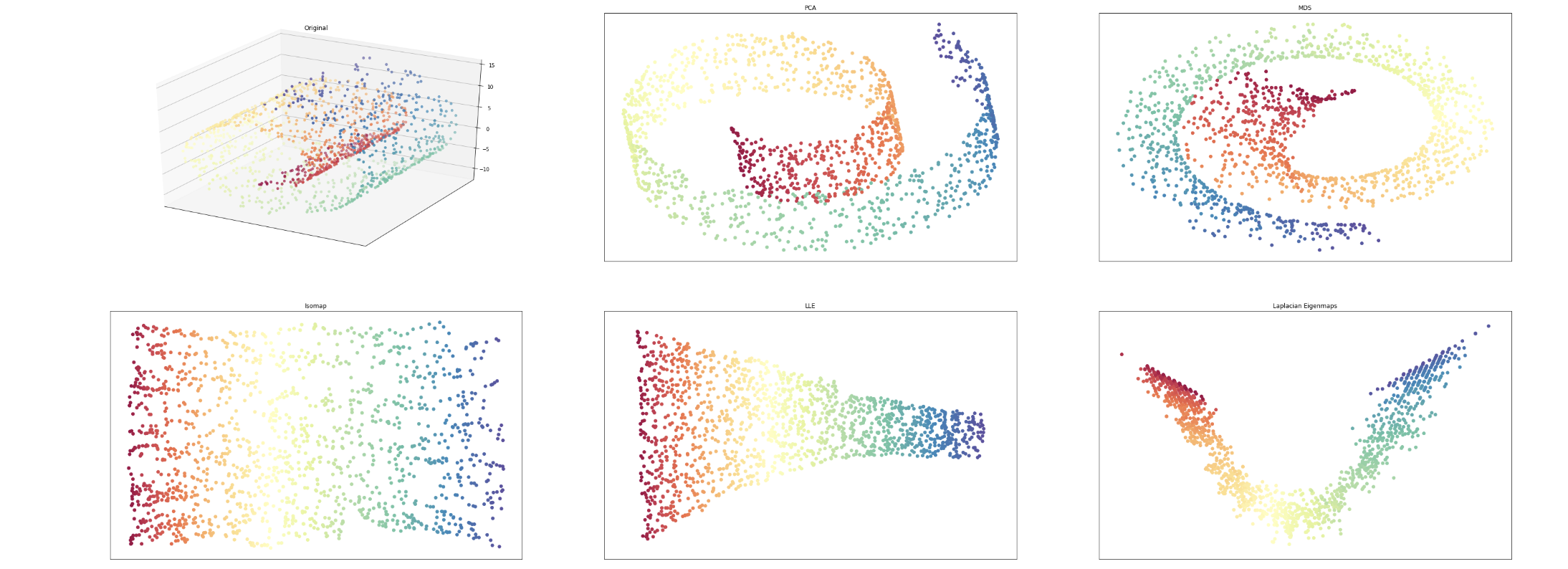
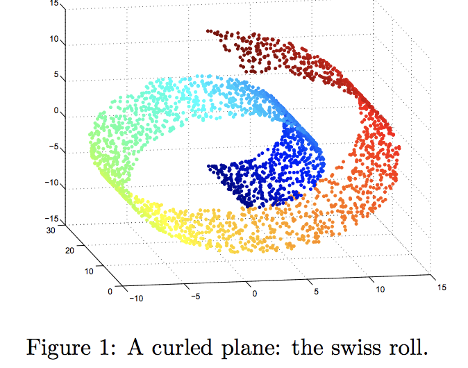
PCA has been very successful in a lot of dimensional reduction tasks. For example latent semantic analysis mentioned earlier uses PCA, population structure in the genetic data from different geographical locations can be inferred using PCA etc. Despite it’s popularity, PCA has some obvious shortcomings, most notably is the assumption that data lie on a linear subspace. If the data lie along a curled plane, e.g. a swiss roll embedded in 3-dimensioanl Euclidean space, PCA wouldn’t be able to find the 2-dimensional representation even though the data is obviously 2d.
Remark This is true for any symmetric, non-negative with zeros on the diagonal.
The spectral decomposition of the Gram matrix of \(X\) gives - \[X^T X = U \Lambda U^T\] Thus the optimization becomes minimization of \[|| U \Lambda U^T - \hat{X}^T \hat{X}||\] which can be solved by \[\hat{X} = U \Lambda^{1/2}\] To obtain a low-dimensional embedding in \(d\)-dimensions, take only top \(d\) eigenvalues and their corresponding eigenvectors of \(X^T X\) i.e. top values of \(\Lambda\).
Proposition MDS prodecure for Euclidean distance matrix is equivalent to the PCA.
Proof: If \(\hat{X} = U \Lambda^{1/2}_{d}\) is the \(d\)-dimensional embedding obtained from MDS as above, the the spectral reconstruction of the Gram matrix is \[X^T X = U \Lambda^{1/2}_{d} U^T\] Also the projection of \(X\) onto top \(d\) principal components is \(P = XV\), where \(V\) is made of eigenvectors of \(X^T X\). If \(v_i\) is a column of \(V\) (i.e. eigenvectors of \(X^T X\)) \[\begin{aligned} X^T X v_i = \sigma_i v_i \\ (U \Lambda^{1/2}_{d} U^T)^T (U \Lambda^{1/2}_{d} U^T) v_i = \sigma_i v_i \\ ( \Lambda^{1/2}_{d} U^T U \Lambda^{1/2}_{d}) = \sigma_i v_i \\ \Lambda^{1/2}_{d} v_i = \sigma_i v_i\end{aligned}\] Thus \(v_i\) is the \(i\)th standard basis vector for \(\mathbb{R}^{D}\). \[P = XV = X <v_i>_{i=1}^{i=d}\] Thus the truncation in MDS is equivalent to projecting X onto its first d principal components.
Remark The above discussion is true only for Euclidean distance matrix. In practice, the distance matrix can express any type of dissimarities between the data points.
Manifold learning methods can be thought of a non-linear generalization of PCA, where the data in no longer assumed to lie on a linear subspace. Instead we assume that the data lie on a low-dimensional manifold embedded in the feature space.
Definition: Let \(U \subset \mathbb{R}^{n}\) and \(V \subset \mathbb{R}^{k}\) be open sets, and \(f : U \rightarrow V\) be a function. Then \(f\) is smooth if all of the partial derivatives of \(f\) are continous. i.e. for any \(m\) \[\frac{\partial^{m}f}{\partial x_i \ldots \partial x_m} \hspace{5mm} \text{is smooth}.\]
We have not rigorously defined open sets in a topological space (e.g. \(\mathbb{R}^{n}\)), intuitively they are extensions of open intervals on real line. And we don’t need the notion of continuity of a function in its full glory. In this article, we are restricting to sets in Euclidean spaces.
Smoothness of a function can be extended to arbitrary sets (not necessarily open) as follows.
Defintion: Let \(X \subset \mathbb{R}^{n}\) and \(Y \subset \mathbb{R}^{k}\) be arbitrary subsets. A function \(f : X \rightarrow Y\) is smooth if for each \(x \in X\), there exists an open neighborhood \(U \subset \mathbb{R}^n\) and a smooth function \(F: U \rightarrow \mathbb{R}^k\) that coincides with \(f\) on \(U \cap X\).
Definition: A function \(f : X \rightarrow Y\) is a homeomorphism if it is a bijection of sets with both \(f\) and \(f^{-1}\) continous. A homeomorphism is called a diffeomorphism if both \(f\) and \(f^{-1}\) are smooth.
Equipped with this terminology, we are now ready to define a manifold. A manifold is a topological space which is locally diffeomorphic to some Euclidean space. To be more precise,
Defintion: Let \(M \subset \mathbb{R}^{n}\), then \(M\) is a smooth manifold of dimension d if for each \(x \in M\), there exists an open neighborhood \(U\) containing \(x\) and a diffeomorphism \(f: U \rightarrow V\) where \(V \subset \mathbb{R}^{d}\).
These open neighborhoods are called the coordinate patches and the diffeomorphisms are called coordinate charts.
Consider the example of a dataset shown in the Figure 1, commonly referred to as swiss roll. It is clearly 2-dimensional embedded in 3-dimensional Euclidean, but is not a linear subspace. PCA would not be able to correctly decipher the underlying structure. The swiss roll is actually a 2-dimensional submanifold of the Euclidean space. This and many such example ask for a more general framework for dimensional reduction where we disband the linear subspace requirement (as in PCA) to capture the non-linearities in the dataset.
Based on previous discussions, we need to move to the next general category of spaces1. To extract linear subspaces, e.g. in PCA, we work in the category of vector spaces over the field of real numbers. These spaces are globally flat (no curvature). In fact, all the datasets we would encounter will be subsets of Euclidean spaces (\(\mathbb{R}^n\)). The next step in abstraction is to lift to the category of locally flat spaces i.e. the spaces which look like vector spaces locally. Mathematically this is the category of manifolds embedded in \(\mathbb{R}^n\) and it includes vector spaces over reals as a subcategory. In the same spirit, we look for submanifold embeddings of original data manifold.
Every real vector space is a real manifold, so we should be able to extract the linear subspace structure in case such a situation presents itself.
For more curious, there is a more general category of spaces called topological spaces and there is a very active of research called topological data analysis, where the data points are assumed to be sampled from a topological space. This is the most general category of mathematical spaces that the author is aware of. Evidently TDA has shown great progress in unraveling hidden structure in variety of datasets.
Schematically, \[Vect_{\mathbb{R}} \subset Manifolds_{\mathbb{R}} \subset Top_{\mathbb{R}}\]
In this article, we will be working with datasets with finite points, which are assumed to be sampled from an infinite space e.g. a manifold or a vector space. The goal is to learn the properties of the manifold from the sample points.
Isometric Mapping (Isomap) is one of the earlies manifold learning methods, which can be thought as a non-linear extension of the MDS. The idea to perform MDS in the geodesic space of the underlying manifold instead of the distance matrix of the Euclidean space. A geodesic is a generalization of the concept of a straight line to curved manifolds, which defines the shortest path between two points on a manifold along its curved geometry.
Maintaining the syntax of the above discussion, the data is drawn from a \(d\)-dimensional manifold \(M\) embedded in \(\mathbb{R}^D\) and we hope to find its coordindate charts \[f : M \to \mathbb{R}^d\] Isomap assumes that the coordinate chart is an isometry i.e. preserves the geodesic distance between points. If \(G(x_i, x_j)\) is the geodesic distance between two points \(x_i, x_j\) on M, then \[|| f(x_i) - f(x_j)|| = G(x_i, x_j)\] Isomap procedure comprises of the following steps:
Compute the pairwise geodesic distances between data points.
Perform MDS on geodesic matrix to map data points onto a low-dimensional space.
The optimization problem can be defined as follows:
Given a data sample \(X = \{ x_1, x_2, \ldots, x_n \} \subset M \subset \mathbb{R}^{n \times D}\) of \(D\)-dimensional points, find an embedding \(f:M \to \mathbb{R}^d\) such that \[min \sum_i \sum_j [G(x_i, x_j) - D(f(x_i), f(x_j)) ]^2\] where \(G\) is the geodesic distance and \(D\) is the Euclidean distance.
To compute geodesic distances between points on a finite set, we define a nearest neighbor graph of the data. This graph has every data point as a node and an edge is defined from node \(x_i\) to \(x_j\) if \(x_j\) is one of the \(k\)-nearest neighbors of \(x_i\). We define nearest neighbors in the high-dimensional Euclidean space. In some settings, one can also define the neighborhood graph consisting of all the points within some radius \(\epsilon\). Each edge is weighted by the Euclidean distance between the nodes. \[G = \{(x_i,x_j,w_{ij}) | w_{ij} = ||x_i - x_j|| < \epsilon \}\] Having constructed the neighboorhood graph of the data, we define the geodesic distance between two points as the shortest-path distances betwen them on this graph, which can be computed by e.g. Dijkstra’s or Floyd’s algorithm. \[g(x_i, x_j) = \text{shortest-path distance}_{G}(x_i, x_j)\]
Equipped with the notion of geodesic distance between two points, we build the affinity matrix containing the pairwise geodesic distances between the data points. \[(\mathcal{G})_{ij} = (g(x_i, x_j))\] The Isomap algorithm proceeds to compute embeddings by employing the MDS procedure on the distance matrix \(\mathcal{G}\). As discussed above, the distance matrix \(\mathcal{G}\) can be converted to the Gram matrix \[X^T X = \frac{1}{2} H \mathcal{G} H\] which then be diagonalized to obtain \[X^T X= U \Lambda U^T\] and \(d\)-truncation, \(\hat{X}_d = U \Lambda^{1/2}_{d}\), obtained by restricting to top \(d\) entries of \(\Lambda\) and the corresponding enties of \(U\), gives a \(d\)-dimensional embedding of the data matrix \(X\).
It can be shown that in a large enough sample, the graph distances approximate the original underlying geodesic distances if the following are true:
The manifold is compact.
The coordinate chart is an isometry.
The underlying parameter space (i.e. the image of the inverse coordinate chart function \(f^{-1}: \mathbb{R}^d \to M\)) is convex.
The manifold is well sampled everywhere.
This can be used to prove that Isomap is guranteed to find the optimal solution. For explicit mathematical details, see Graph approximations to geodesics on embedded manifolds, 2000.
Identify the neighbours of each data point \(x_i\).
Compute the weights that best linearly reconstruct \(x_i\) from its neighbours.
Find the low-dimensional embedding vector \(\hat{x}_i\) which is best reconstructed by the weights determined in the previous step.
The neighborhood set for a data point \(x_i\) can be defined as the set of k-nearest neighbors \[N_k(x_i) = \{ x \in X |\text{$x$ is a k-nearest neighbour of $x_i$} \}\] LLE assumes that each data point \(x_i\) can be reconstructed from its nearest neighbors \(N_k(x_i)\) as a weighted, convex combination. \[\hat{x}_i = \sum_{j \in N_k(x_i)} W_{ij}x_j\] The weights \(W_{ij}\) describe the local geometry of the neighborhoods. The weights are obtained by minimizing the error: \[|| x_i - \hat{x}_i||^2 = ||x_i - \sum_{j \in N_k(x_i)} W_{ij}x_j ||^2\] Each row in the weight matrix should sum to one (convex combination) and \(W_{ij} = 0\) if \(j \notin N_k\). It’s evident that the weight matrix is invariant to the global translations, rotations and scalings.
For a data point \(x\), the error we want to minimize is \[E = ||x - \sum_{j \in N_k(x)} W_{j}x_j ||^2\] which can written as (since \(\sum_{j \in N_k(x)} W_{j} = 1\)) \[||x_i - \sum_{j \in N_k(x)} W_{j}x_j ||^2 = || \sum_{j \in N_k(x)} W_{j}(x - x_j) ||^2 = \sum_{jk}W_{j}W_{k}G_{jk}\] where \(G_{jk} = (x - x_j) . (x - x_k)\) is the Gram matrix, which is symmetric and semi-positive definite. The optmization has a closed form solution using Largange mulitplier for the constraints: \[W_{j} = \frac{\sum_k G^{-1}_{jk}}{\sum_{lm}G^{-1}_{lm}}\]
Since the weight matrix (local geometry) corresponding to a data point \(x\) is invariant to translation, rotation, and scaling, it should be preserved in any linear mapping of the neighborhood around \(x\). In particular, the weight matrix should also describe the local geometry of the image of the cooridinate chart (parameter space) containing \(y = f(x) \in \mathbb{R}^d\). Thus, the optimal \(d\)-dimensional embedding is the one that constructs \(y\) from its nearest neighborhood using the same weights that we estimated above. We will minimize the error function \[e = \sum_i || y_i - \sum_j W_{ij} y_j||\] with respect to \(y_i \in \mathbb{R}^d\).
The error function can be expressed in the matrix form as \[e = Y^T M Y\] where \[M_ij := \delta_{ij} - W_{ij} - W_{ji} + \sum_k W_{ki} W_{kj}\] with constraints \[\begin{aligned}
\sum_i Y_i = 0, \text{fix translational degree of freedom in the error function.} \\
Y^TY = I, \text{fix rotational degree of freedom in error, and to fix scale.} \\\end{aligned}\] The error function in this form resembles the Rayleigh quotient (defined for any matrix \(M\) and a vector \(x\) as \(x^T Mx / x^T x\)).
For any matrix \(M\) and vector \(x\), the Rayleigh quotient \(x^T Mx / x^T x\) is minimum at the smallest eigenvalue of \(M\) and the vector \(x\) is corresponding eigenvector.
Using the above, the error functiion \(Y^T M Y\) can be minimized by setting the columns of \(Y\) to be eigenvectors of \(M\) corresponding to the smallest \(d\) eigenvalues. However, the smallest eigenvalue is 0 which corresponds to identity eigenvectors, thus the \(d\)-dimensional embedding is obtained by taking smallest non-constant eigenvectors.
For reference, orginal paper - Think Globally, Fit Locally: Unsupervised Learning of Low Dimensional Manifolds
Simplified binary weighting. \[W_{ij} = \begin{cases} 1, \quad\text{if} \quad x_j \in N(x_i)\\ 0, \quad\text{otherwise} \end{cases}\]
Weighting by the Gaussian heat kernel \[W_{ij} = \begin{cases} e^{- ||x_i - x_j||^2 / 2\sigma^2}, \quad\text{if} \quad x_j \in N(x_i)\\ 0, \quad\text{otherwise} \end{cases}\] This requires a choice for the value of \(\sigma\), which is a parameter of this scheme,
This weighting captures the local affinity i.e. a measure of how close the points are to each other. We want to map the weighted graph to a low-dimensional space so that the nearby points stay as close as possible. If \(Y = \{ y_1, y_2, \ldots , y_n \}\) are images of the data points \(X = \{ x_1, x_2, \ldots , x_n \}\) under the (coordinate) mapping, the cost function that we minimize is the following: \[E = \frac{1}{2} \sum_{ij}W_{ij}(y_i - y_j)^2\] This can be expanded as \[E = \sum_{ij}(y_i^2 + y_j^2 - 2y_i y_j)W_{ij} = \sum_{i}y_i^2 D_{ii} + \sum_{j}y_j^2 D_{jj} - 2 \sum_{ij} y_i y_j W_{ij} = 2 y^T (D - W) y\] where \(D_{ii} = \sum_{j}W_{ji}\) is the diagonal weight matrix. The cost function finally can be expressed as \[E = y^T L y\] Where \(L\) is the Laplacian of the graph is defined at \(L := D - W\). The Laplacian is a symmetric and positive semidefinite matrix.
The optimization problem is the the minimization of \(y^T L y\) with constraint that \(y^TDY =1\) which fixes the scale of \(y\). Introducing the Lagrange multiplier, \[y^T L y - \lambda y^TDY = 0 \\\] Thus the vector \(y\) that minimizes the cost function \(E\) is given by the the eigenvectors corresponding to the minimum eigenvalues of the eigenvalue problem \[Ly = \lambda D y\] To obtain a \(d\)-dimensional embedding of \(X\), take the eigenvectors corresponding to the smallest \(d\) eigenvalues avoiding the trivial solution (identity vector for eigenvalue 0).
The Laplacian of a graph has a geometric interpretation as Laplace-Beltrami operator on manifolds. Consider a smooth \(d\)-dimensional Riemannian manifold \(M \subset \mathbb{R}^n\). The Riemannian structure on a manifold can be thought of existence of a notion of metric. If there is a real-valued function on this manifold \[f: M \to \mathbb{R}\] then the gradient of this function \(\Delta f\) defines a vector field on the manifold. In fact a vector field on a manifold is defined by the gradients of the real-valued functions. \[|f(x + \delta x) - f(x)| \sim |< \Delta f, \delta x>| \leq ||\Delta f|| ||\delta x||\] Thus for points closer to \(x\) to be mapped to points closer to \(f(x)\), the \(||\Delta f||\) should be small. Thus the optimization problem becomes:
Find a function \(f\) which is the minima of \[\int_M ||\Delta f||^2\] This translates to finding the eigenvalues of the Laplace-Beltrami operator \(\mathcal{L}\), defined as \[\mathcal{L} = div (\Delta f)\] where \(div\) is the divergence. The Stoke’s theorem that \[\int_M ||\Delta f||^2 = \int_M \mathcal{L}(f) f\] Since \(\mathcal{L}\) is a positive semi-definite, the \(f\) that minimizes the above cost function has to an eigenfunction of \(\mathcal{L}\). This minimization directly corresponds to the minimization of \(Lf = \frac{1}{2} \sum_{ij}(f_i - f_j)^2 W_{ij}\) on a graph.
One of the closely related concepts to the theory of Laplace-Beltrami operator is the heat kernel, which describes the evolution of temperature in a region whose boundary is at a fixed temperature, such that an initial unit of energy is placed at a point at time \(t=0\). The heat kernel is the fundamental solution of the heat equation: \[\frac{\partial u}{\partial t} - \alpha \Delta^2 u = 0\] where \(u: M \to \mathbb{R}\), and \(t\) is the time variable.
This can be written in terms of the Laplace-Beltrami operator as \[\frac{\partial u}{\partial t} - \alpha \mathcal{L} u = 0\] This can be solved as \[u(x,t) = \int_M H_t(x,y) f(y)\] where \(H_t\) is the heat kernel. Thus the optimization (eigenvalue) problem becomes: \[\mathcal{L} f(x) = \frac{\partial}{\partial t} \big( \int_M H_t(x,y) f(y) \big)\] It can be shown that locally the heat kernel is approximated by \[H_t(x,y) \sim (4 \pi t)^{-\frac{n}{2 \pi}}\exp( - \frac{||x-y||^2}{4t})\] where \(||x-y|| <<< \). Also \[lim_{t \to 0} \int_M H_t(x,y) f(y) = f(x)\] For small \(t\) \[\mathcal{L} f(x) \sim - \frac{1}{t} \big[ f(x) - \frac{1}{k}(4 \pi t)^{-\frac{n}{2 \pi}} \int_M \exp( - \frac{||x-y||^2}{4t}) f(y) dy \big]\] where we have put \(\alpha = \frac{1}{k}(4 \pi t)^{-\frac{n}{2 \pi}}\). Since Laplacian of a constant function is zero, we get \[\frac{1}{\alpha} = \sum_{y, ||x - y|| < \epsilon} \exp( - \frac{||x-y||^2}{4t})\] We approximated the integral by the summation over the \(\epsilon\) neighborhood. Thus to translate the ideas from manifold operator theory to the spectral graph theory, we see that the weights for the edges to be chosen as
\[W_{ij} =
\begin{cases}
e^{- ||x_i - x_j||^2 / 4t}, \quad\text{if} \quad x_j \in N(x_i)\\
0, \quad\text{otherwise}
\end{cases}\] For references, see Laplacian Eigenmaps and Spectral Techniques for Embedding and Clustering.